TDMM: Bayesian Time-Dynamic Models with Optional Mixed Effects fits Gaussian, Bernoulli, and Poisson responses with regression coefficients that vary smoothly over time. With random_intercept = TRUE (the default), a subject-specific random intercept supports repeated observations at irregular times and unequal visit counts. With random_intercept = FALSE, the model supports independent observations; time may represent age, time since an event, or time relative to an event. With repeated observations, numeric covariates can be constant within subject or change at each visit. The default is eight cubic B-spline basis functions (degree 3, order 4) with a second-order coefficient-difference penalty. Install JAGS before fitting.
This page accompanies the package’s Getting Started vignette.
Data and fitting
Provide one row per observation, with columns for subject ID, numeric time, response, and covariates. The order of x.var determines the coefficient labels: beta1 multiplies the first covariate, beta2 the second, and so on. The following Gaussian fit demonstrates repeated observations and uses random_intercept = TRUE.
library(TDMM)
fit <- tdmm(long_data, family = "gaussian",
            subject.var = "id", time.var = "time", y.var = "y",
            x.var = c("baseline", "changing"), n_basis = 8,
            random_intercept = TRUE,
            control = tdmm_control(chains = 3, iterations = 4000,
                                   burn_in = 1500, thin = 2,
                                   adapt = 2000, seed = 77181),
            priors = tdmm.priors("gaussian"))
summary(fit)
plot(fit)
plot.trace.tdmm(fit, c("sigma.b", "sigma2.e", "tau.alpha[1]"))
Here baseline should be repeated within subject and changing may vary by visit. TDMM handles the subject indexing and spline construction. The Gaussian coefficient curves are on the response scale; Bernoulli coefficients are on the log-odds scale and Poisson coefficients on the log-mean scale. Inspect trace plots, R-hat, effective sample size, and credible bands before interpretation.
For independent observations, use random_intercept = FALSE to omit the subject-specific random intercept.
Coefficient-function recovery
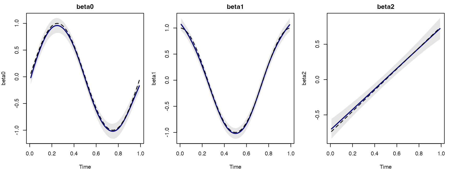
The figure illustrates coefficient-function recovery for a simulated repeated-observation Gaussian study fit with random_intercept = TRUE. Solid lines show posterior means, dashed lines the truth, and shaded regions pointwise 95% credible bands. The repeated-observation section of the Gaussian examples shows the corresponding fitting workflow. The Gaussian, Bernoulli, and Poisson example pages also include independent-observation workflows using random_intercept = FALSE.
PBC2 real-data application
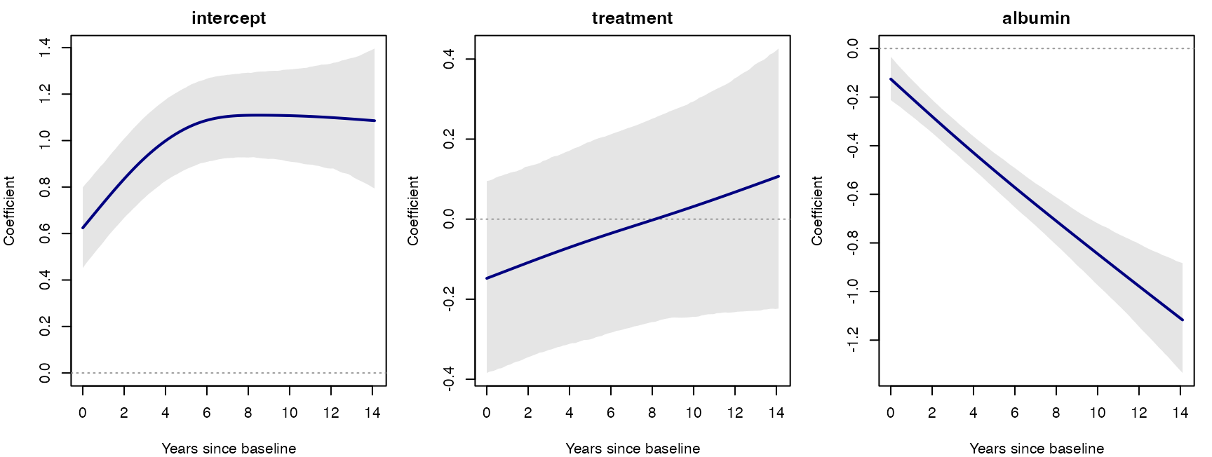
The PBC2 application uses the pbc2 dataset from JMbayes2: 1,945 observations from 312 subjects, with 1–16 visits. The response is log serum bilirubin; predictors are a baseline treatment indicator and longitudinal albumin. Albumin is centered at its overall observation-level mean, 3.3898868894601542 g/dL. Thus the intercept represents the modeled placebo trajectory at that albumin level and random intercept zero.
The treatment 95% credible interval includes zero throughout the common evaluation grid. The albumin coefficient is negative, with its band below zero on that grid. These are conditional associations, and the treatment curve does not establish a causal effect. Late follow-up is sparse, so small tail fluctuations should not be read as precise clinical changes.
Using your own data
First determine whether your data contain repeated observations or independent observations. For repeated observations, use random_intercept = TRUE (the default) to include a subject-specific random intercept; subject IDs may appear on multiple rows. For independent observations, use random_intercept = FALSE; each subject contributes one observation, and time may represent age, time since an event, or time relative to an event. Then choose family = "gaussian", "bernoulli", or "poisson" and supply the intended covariates in x.var order.
The data checks reject missing analysis values; decide how to handle missingness before fitting. Varying n_basis is a useful sensitivity check; scientifically important smoothing or variance priors can also be examined using tdmm.priors(). To run MCMC chains in parallel on macOS or Linux, use tdmm_control(parallel = TRUE, cores = 2, ...).